Simulation of physical systems using digital computers has been accomplished by many people over the past few years. One such simulation program at Cornell Aeronautical Laboratory, Inc. constitutes an analytical representation of an automobile as it departs from the highway under various environmental conditions, especially under adverse ones where there is danger of collision with obstacles [1]. As with most complex simulation programs where there are interactions among many components, the equations of motion, including the required restraints, become long and numerous. But foremost, the output data set in printed form is quite extensive and very difficult for the investigating engineer to completely comprehend. About thirty crowded pages of output are printed for a five second automobile test run.
The objective of the task described here was to convert some of these output data into a pictorial form; that is, pictures were desired for a simulated automobile undergoing various violent maneuvers. In this manner, the actions in any part of the vehicle can be easily and quickly determined. Since this objective could be applied to most simulation problems to advantage, a set of generalized computer subroutines were designed to be called in a manner similar to most plotting utility packages.
The pictures are then drawn by state-of-the-art peripheral plotting hardware. Several output methods are available to CAL users:
The CAL Single Vehicle Accident Program [1] simulates a moving automobile, its interaction with the terrain over which it travels and collisions with a variety of obstacles in its path. The program is very flexible in that approximately 100 input parameters describe the automobile, such as wheel base, weight, braking coefficients, nonlinear characteristics of shock absorbers, engine torque on driver wheels, etc. Likewise, various terrain profiles and obstacles can be specified for different simulation runs. For example, the radial tire force generated at each wheel is simulated by means of simple springs on smooth terrain; however, on rough terrain or when obstacles, such as curbs, are encountered, the tires are simulated by a set of compound springs radiating from the hub of the wheel. Originally, the output consisted of about sixty items of response printed in tabular form.
For a first effort at pictorial output, the automobile is considered as four different objects, namely, the two front wheels, the rear axle and the sprung mass (the body). The Single Vehicle Accident Program was modified to record dynamically on magnetic tape thirteen parameters which describe the actions of these four objects. They are:
1-3    position of the sprung mass,
4-6    attitude of the sprung mass,
7-8    deflection of each of the front wheels,
9-10   camber of each of the front wheels,
11     deflection of the rear axle,
12     roll of the rear axle,
13     steer angle applied to the front wheels.
This magnetic tape is the dynamic input to the picture generation program. Other objects, such as road markings, roadside barriers, ramps, etc., are static initial inputs to the program.
A quick but incomplete review of the available literature revealed that a number of different approaches to producing three-dimensional computer graphics displays have been developed [2][3][4] [5]. However, none met our particular requirements to permit quick economical generation of both still and motion pictures with the existing in-house equipment available.
The pictures are drawn as line drawings using straight lines only. The periphery of a wheel, for example, is drawn as a 50-sided regular polygon. No attempt was initially made for hidden line removal.
Each object is stored as one or more three-dimensional arrays; each entry defines a point of the object with respect to three-dimensional rectangular coordinates fixed in the object. Thus, after the appropriate coordinate transformations discussed below, a perspective picture can be drawn in two-dimensional space by starting at the first point of the first array, drawing a straight line to the second point and proceeding onto each point of the array in turn. This is done for each array of the object.
The usual description of a simple pinhole camera as illustrated in Figure 1 is used. The position of the image, Q, on the picture plane of an object at point P in front of the camera with a focal length of F is:
(1)    xQ = 0
(2)    yQ = -F yp/(xp - F)
(3)    zQ = -F zp/(xp - F)
Thus, the three-dimensional space in front of the camera is mapped onto the two-dimensional space of the picture plane (film) of the camera. The simulation of this simple camera is the crux of our picture generating program.
In addition, care must be taken to assure that attempts are not made to draw portions of the object image which are outside the picture boundary. At first thought one might expect this to occur only when
(4)    |yQ| ≥ Ymax
or
(5)    |zQ| ≥ Zmax
Actually this occurs also as
(6) xp - F → -
For drawing a single straight line, only the central portion, an end, or the whole line may be in view. Thus, intersections of lines and picture edges must be continually tested. For example, see Figure 2.
Line AB is defined in the object array by points A and B, the transformations of both lie outside the picture. However, the central portion of the line lies inside the boundary and must be drawn. Thus, for lines where at least one of the end points lies outside the boundary, algorithms were developed to determine which portion, if any, of the line is to be drawn.
As noted above, coordinate transformation of the arrays of points of an object in three-dimensional space to points of the picture in two-dimensional space is necessary. This is done with the help of the following coordinate systems and relating parameters.
Motion and dynamic activity in the simulated scene to be photographed is reflected in changes over time of the position and attitude parameters (a total of six) for each object. Furthermore, change in the camera parameters are also possible. The camera could be mounted on a vehicle. Panning (attitude changing) and/or zooming (changes in focal length) are included.
Consider a point of an object, any point in the object description arrays, as a row vector, P0, described in object space. The position vector with respect to inertial space, is obtainable by the transformation.
(7) PI = P0 × [OI] + B
where the transformation matrix is
               |cosPcosY, sinPcosYsinR - cosRsinY, sinPcosYcosR + sinRsinY  |
               |
(8)    [OI] =  |cospsinY, sinPsinYsinR + cosRcosY, sinPcosYcosR - sinRcosY  |
               |
               |   -sinP, cosPsinR               , cosPcosR                 |
Similarly, in camera space, the relationship is
(9) Pc = (PI - C) × [IC]
where the transformation is
               ! cosA cosE    ,  sinAcosE,  sinE |
               |                                 |
(10)    [IC] = |  -sinA       ,   cosA   ,   0   |
               |                                 |
               | -cosAsinE    , -sinAsinE,  cosE |
At this point the value of the x component of Pc, Xpc, is checked. If Xpc ≤ F (see Figure 1), the point is (1) behind the camera, or (2) at the camera focal point, or (3) its corresponding picture image point will be a very large distance from the center of the picture, i.e., xQ, yQ→∞. Thus, complete lines connecting to the point cannot be drawn.
The final transformation to the two-dimensional point in the picture plane is
(11) Q = KF/(Xpc-F) Pc× [CP]
where K is an enlargement factor and the transformation matrix is
               |   0   ,   0   |
               |               |
(12)    [CP] = | -cosT , sinT  |
               |               |
               |  sinT , cosT  |
Now the point must be checked to determine whether it is within the picture frame by the following criteria:
(13)    | xQ ≤ W/2

(14)    | yQ ≤ H/2
where W and H are the prescribed width and height of the picture, respectively.
The program was written using the FORTRAN IV source language and documented for general usage in the analysis of automobile dynamics.
The subroutines were designed to supply the rudimentary requirements for drawing perspective line drawings. A brief description of each subroutine call follows.
The executive routine reads the magnetic tape describing the thirteen parameters of the automobile dynamics. These in turn are used for determining the spatial relationships of the object coordinates for each of the four objects (the two front wheels, rear axle and sprung mass) of the automobile for each increment in time. Calls to the picture subroutines are then made to draw the pictures. Background objects such as road markings, barriers, ramps, etc., are read in from cards. Other features of the program include:
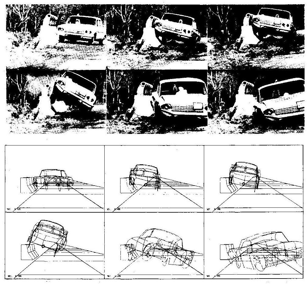
Sample still pictures from several different simulated vehicle maneuvers are shown in Figure 4, Figure 5 and Figure 6, together with pictures of similar real life tests. Automatic panning is used in all cases.
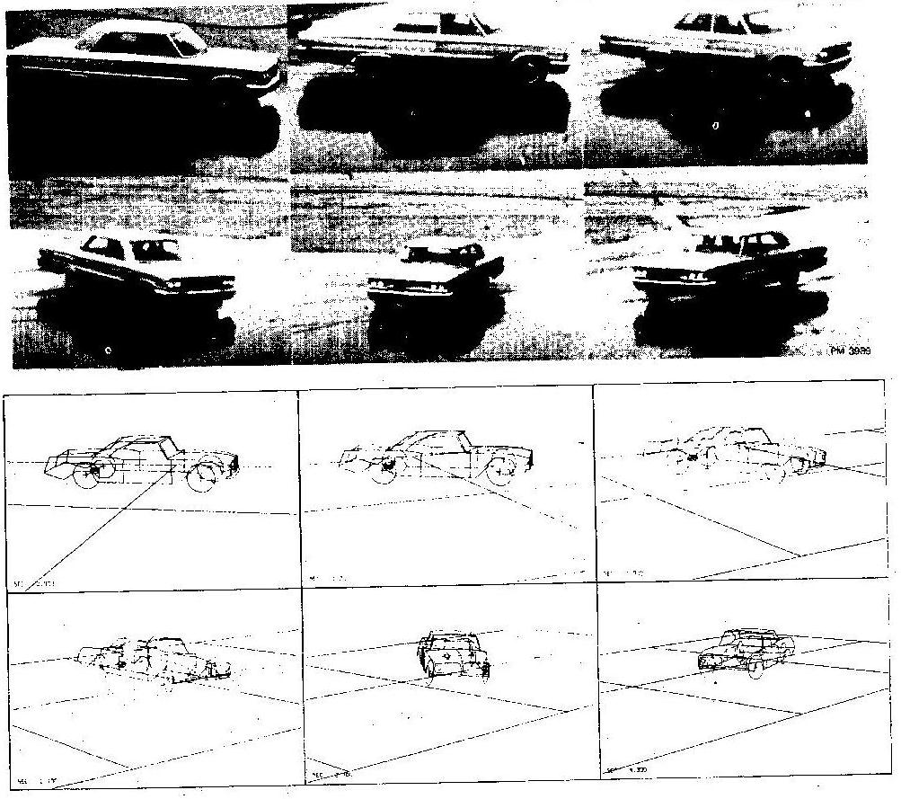
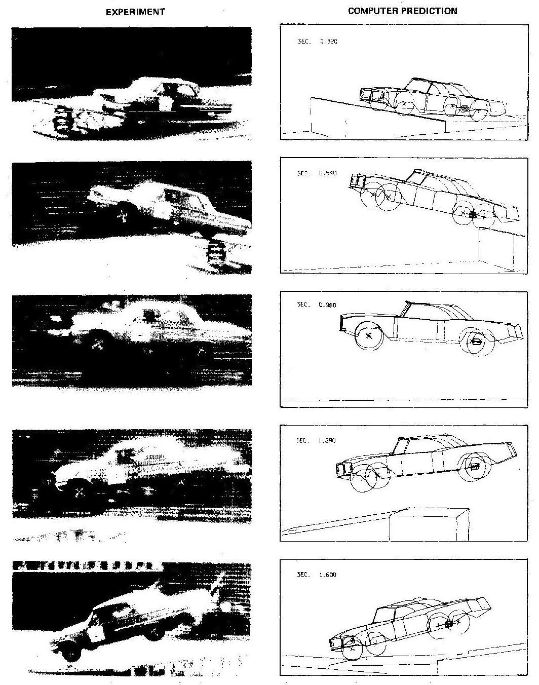
The pictures illustrate the ease of assessing the capability of the simulation program. Through comparisons with similar real life test pictures, especially motion pictures, one may quickly verify the validity of a simulation program and establish a high degree of confidence in its usage.
These results encourage one to look ahead to future activity. The various other applications of this output technique to simulation is limited only by the user's imagination and needs. Improvements, of course, are desirable. First of all, the removal of hidden lines would improve the esthetic value. The literature contains several methods of varying levels of satisfying and financially feasible results [7] [8] [9]. The economical inclusion of color and shading is challenging. Illustration of the deformation of objects, such as the crushing of an automobile fender, would be highly desirable.
Figure 5-Photographic and computer graphic display of skidding vehicleI wish to express my gratitude to Raymond R. McHenry and Clarn W Swonger fr their help and guidance in the development work leading to this paper.
The reported research was performed under Contract No. CPR-11-3988 with the Traffic Systems Division, Office of Research and Development, Bureau of Public Roads, U. S. Department of Transportation. The opinions, findings and conclusions expressed in this paper are those of the author and not necessarily those of the Bureau of Public Roads.
1. R R McHenry, N J DeLeys, Vehicle dynamics in single vehicle accidents - validation and extensions of a computer simulation, Cornell Aeronautical Technical Report VJ-2251--V-3 December 1967.
2. K C Knowlton, A computer technique for producing animated movies, AFIPS 1964
3. A M Noll, Computer-generated three-dimensional movies, Computers and Automation November 1965
4. W A Fetter, Computer graphics, Annual Meeting of the American Society for Engineering Educators 1966
5. R L Mitchell, A computerized 3-D plotting program, Computerized Imaging Techniques, Proc of the Society of Photo-Optical Instrumentation Engineers, June 1967
6. C M Theiss, Perspective picture output for automobile dynamics simulations, Cornell Aeronautical Laboratory Technical Report VJ-2251-V-2R, January 1969
7. L G Roberts, Machine perception of three-dimensional solids, Lincoln Laboratory Technical Report 315 May 1963
8. R A Weiss, BE VISION, a package of IBM 7090 FORTRAN programs to draw orthographic views of combinations of plane and quadric surfaces, JACM, April 1966
9. P Loutrel, A solution to the hidden-line problem for computer-drawn polyhedra , New York University School of Engineering Teehnical Report, September 1967 400-167