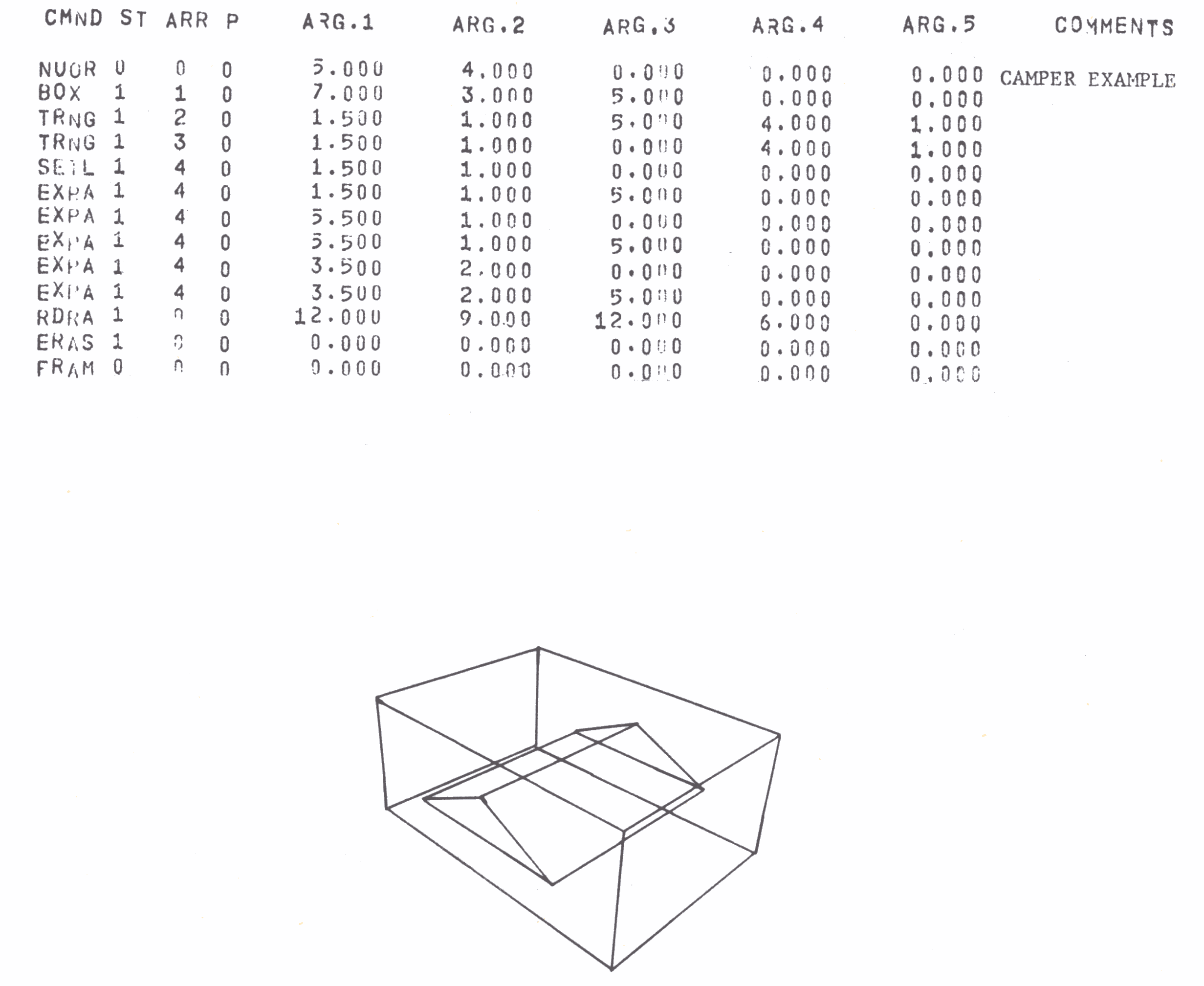
CAMPER (Computer Aided Movie Perspectives) is a program designed and implemented by Sherwood Anderson as part of his MSc Dissertation at Syracuse University. The aim was to produce an efficient picture language for producing computer animated films. This manual derives from a number of papers available on the system (see references at end).
CAMPER is a 3D extension of a 2D system called CAMP. No knowledge of computer programming languages is required. The user produces a set of data cards where each card is a statement in a very simple language. each data card contains all the relevant information needed to describe a particular figure or to perform some operation upon a previously defined figure. The card format consists of a maximum of five letters defining the command followed by a group of numbers located in the appropriate card columns which specify the arguments of the command. the language is planned so that a potential user can quickly design and produce films without guidance.
The basic philosophy is to approximate all picture elements in the film by straight lines. Although curved regions of the figure may suffer, there is considerable economy and simplicity because of this. Only the coordinates of the endpoints of each line are stored. A simple storage structure is used to keep complex pictures in a fairly compact form. Using this, the same picture can be produced repeatedly without wasting time regenerating the points defining each frame. If the user wishes to change only certain parts of a figure, he can easily do so by altering only those points in question in the storage structure.
The storage area is broken down into a number of distinct parts called stacks. Each new figure is added at the end of a stack when it is defined. the individual figures are called arrays. A single command can either operate on a single array or a whole stack. Arrays are numbered and care must be taken to generate them sequentially. For example, a circle might be defined as array 1 in stack 1. this could be followed by a definition of a triangle as array 2 of stack 1 and so on. Arrays can be processed in any order once generated. the contents of an array can be replaced by a second figure providing that it requires the same number of locations (see the Appendix). The 1906A version of CAMPER has an 8000 word area of store defined as 8 stacks of 1000 words.
In general, the user need not know how the arrays are stored in the stacks. However, the information can be quite useful to the more sophisticated user wishing to manipulate and transfer arrays from stack to stack.
Basically an array can be of one of two forms :-
The array consists of pairs of coordinates which define separate lines to be plotted. For example, an array could be X1, Y1, Z1, X1', Y1', Z1', X2, Y2, Z2, X2', Y2', Z2',...
The array consists of a set of point coordinates such as X1, Y1, Z1, X2, Y2, Z2, X3, Y3, Z3,... and this defines a set of line segments from (X1, Y1, Z1) to (X2, Y2, Z2), from (X2, Y2, Z2) to (X3, Y3, Z3) and so on.
It is also possible to have a HYBRID array which starts off in one form and changes form (possibly several times) within the array.
The picture area visible from a normal view point is 0 < X < 12, 0< Y < 9, 0 < Z < 9. Consequently all X,Y,Z variables in the array will be of a similar size to these values. A value greater than 10000 would therefore not be a coordinate value. Five values of this order of magnitude are therefore chosen as data markers to define the type of the array information. These are as follows:-
The last two markers are used to produce hybrid arrays. Thus a stack might contain
40000, X1, Y1, Z1, X2, Y2, Z2, 30000, X3, Y3, Z3, X4, Y4, Z4, X5, Y5, Z5,
40000, X6, Y6, Z6, X7, Y7, Z7, 10000, X8, Y8, Z8, X9, Y9, Z9, X10, Y10, Z10,
20000, X11, Y11, Z11, X12, Y12, Z12, 50000
This is:-
The array 1 is a line joining   (X1,Y1,Z1)    to (X2,Y2,Z2)
The array 2 is the set of lines (X3,Y3,Z3)    to (X4,Y4,Z4)
                                (X4,Y4,Z4)    to (X5,Y5,Z5)
The array 3 is the set of lines (X6,Y6,Z6)    to (X7,Y7,Z7)
                                (X8,Y8,Z8)    to (X9,Y9,Z9)
                                (X9,Y9,Z9)    to (X10,Y10,Z10)
                                (X11,Y11,Z11) to (X12,Y12,Z12)
These are the only arrays stored in this stack.
The number of basic figures defined in the system is limited in order to keep storage requirements to a reasonable size. They fall into basically four classes. The first group consists of simple geometric shapes such as circles, triangles, rectangles, crosses. The second consists of more complex shapes which are frequently required. These include arrows and clocks. The third class is only of interest to electrical engineers. the fourth class is a set of alpha-numeric characters of variable size which can be added to a picture at any position.
All commands must be entered by means of data to the system. The column assignment is as follows:-
| Column(s) | Entry |
|---|---|
| 1 - 5 | Command Name |
| 6 | Stack Number |
| 7 - 9 | Array Number (right justified) |
| 10 | Figure Parameter |
| 11 - 20 | Argument 1 |
| 21 - 30 | Argument 2 |
| 31 - 40 | Argument 3 |
| 41 - 50 | Argument 4 |
| 51 - 60 | Argument 5 |
| 61 - 78 | Comment or Text String |
Arguments 1 to 5 can be placed anywhere within the columns allotted, provided a decimal point is included. A blank argument is read as zero. the array number must be right justified; ie the units digit of the array number must appear in column 9.
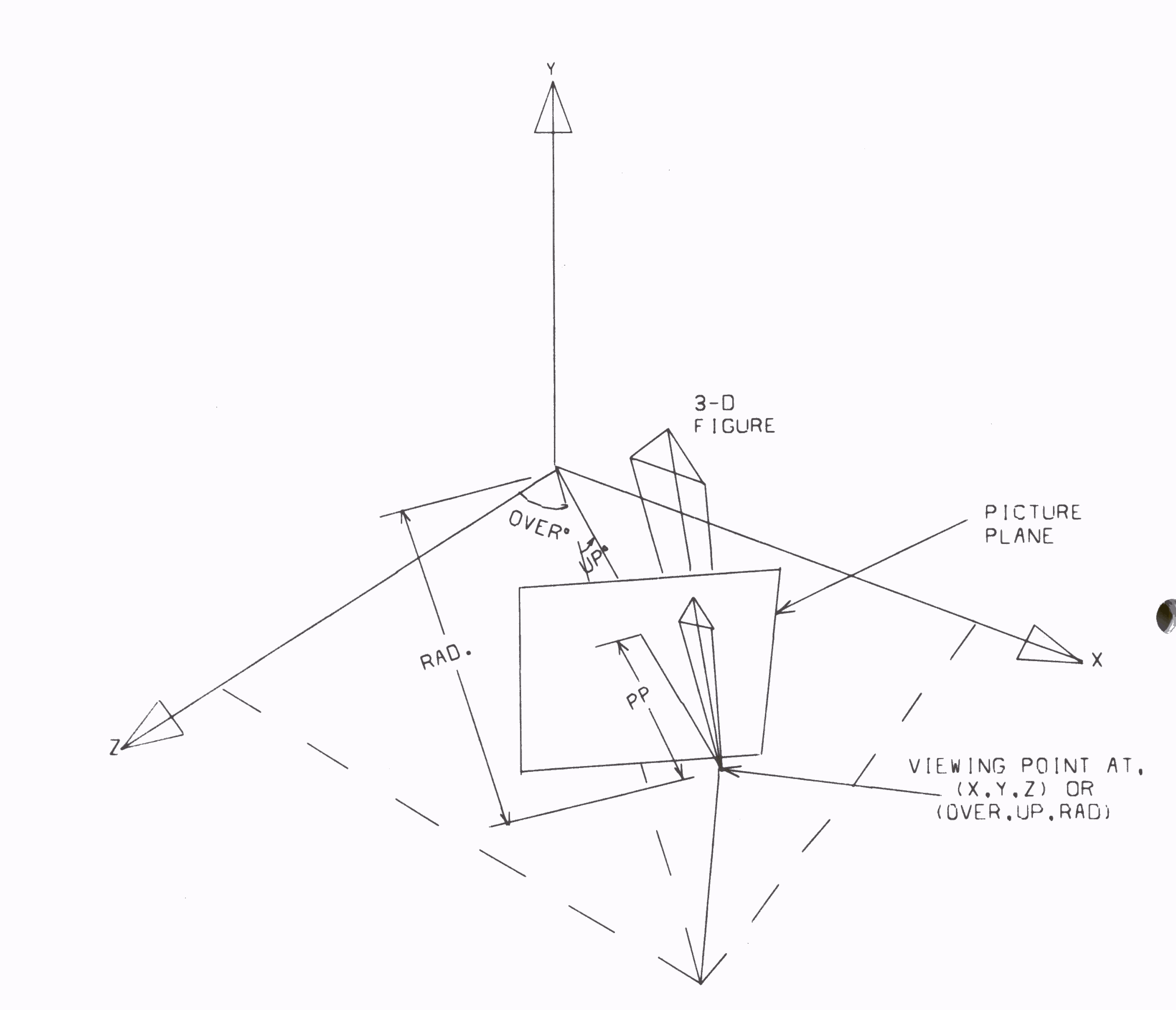
The user defines figures in an area 0 < X < 12, 0 < Y < 9, 0 < Z < 9. A viewing point of this scene is defined as the point (X,Y,Z). Alternatively, the viewing point can be defined in spherical coordinates as (OVER, UP, RAD). Both OVER and UP are given in degrees and RAD is the distance from the origin. A plane can be imagined perpendicular to the line from the viewing point to the origin. This plane is called the Picture Plane. The figure to be plotted normally lies on the opposite side of this plane. Visual rays from the figure to the viewing point pierce the picture plane, tracing out a perspective drawing as it scans the figure. It is this projected view that is calculated by the computer and plotted. The user must define the distance he requires between the viewing point and picture plane. If the picture plane is moved towards the viewer, the image becomes proportionately smaller, and vice versa. The coordinates of the viewing point can be located in any of the eight octants, so that the figure can be observed from any possible position. The following diagram illustrates the geometry.
Before drawing a frame, there is still one parameter to be fixed and that is the part of the picture plane that will be viewed. Initially the perspective point on the picture plane equivalent to the three-dimensional origin is located at the lower left hand corner of the frame drawn. It is possible to change the part of the picture plane that is viewed by defining a new position for the three-dimensional origin.
The list of commands is comprised of 4 basic classes. Class 1 commands set up a figure in an array. the figure must be loaded into an array before it can be drawn. Class 2 commands manipulate the coordinates of an array in some way. Once these commands are invoked, the original array is, of course, destroyed. If it is desired to save these values, they should be transferred into a new array and operated upon there. Class 3 commands perform arithmetic operations upon the 8 variables and define instruction loops. Class 4 commands deal with the plotter itself.
Comments may be placed on every card from columns 61 - 80. However, a special card may be devoted to this purpose by simply putting a C in column 1, comments in columns 61 to 80. Blank commands are ignored. An invalid command ends the program and causes an error message to be printed. All cards are printed out on the users' computer output in the order that they are executed. This is quite helpful when debugging a sequence of commands for a picture.
Commands must always be punched in the format described above. In the text that follows, a less exact format is used with spaces separating the individual fields. A parameter that is not applicable to the command being described is replaced by an asterisk. For example:-
RECT S ARR * X Y Z LNGTH HGT
indicates that the command RECT does not require the figure parameter to be used.
The S and ARR variables always refer to the stack and array to which the picture is being defined.
CIRCL S ARR D X Y Z RAD
defines a circle centred at (X,Y,Z) of radius RAD, in a plane parallel to the x-y plane. If D is nonzero, the circle is dashed. The array is comprised of 37 points, which produces 36 straight lines. the first point lies to the right of the centre, and successive points fall every 10 degrees counter clockwise around the circle.
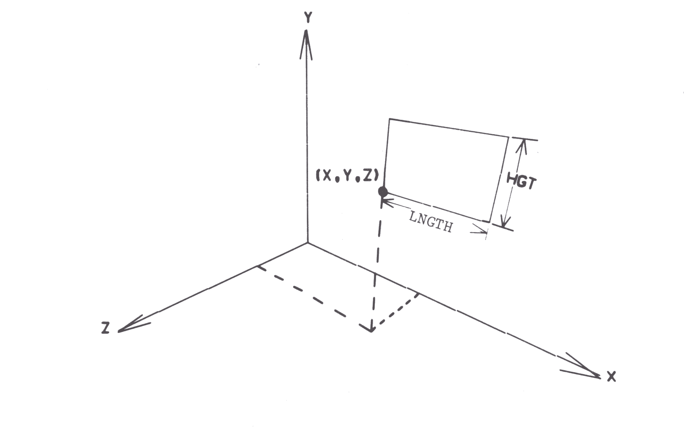
RECT S ARR * X Y Z LNGTH HGT
defines a rectangle with lower left hand corner at (X,Y,Z) of length, LNGTH and height, HGT. This figure lies in a plane parallel to the x-y plane.
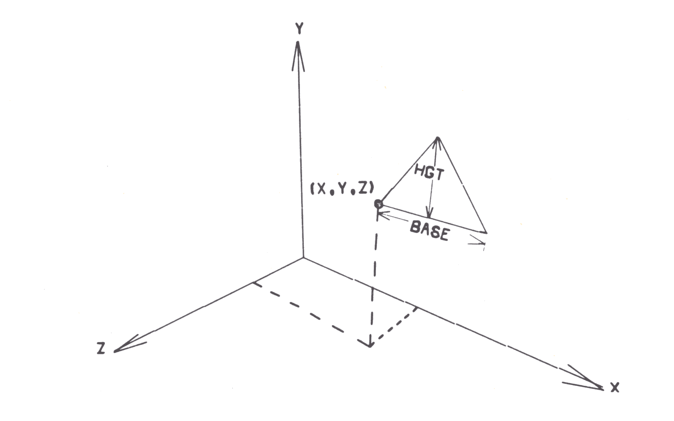
TRNGL S ARR * X Y Z BASE HGT
defines an isosceles triangle with the lower left corner at (X,Y,Z) of base, BASE and height, HGT. The figure lies in a plane parallel to the x-y plane.
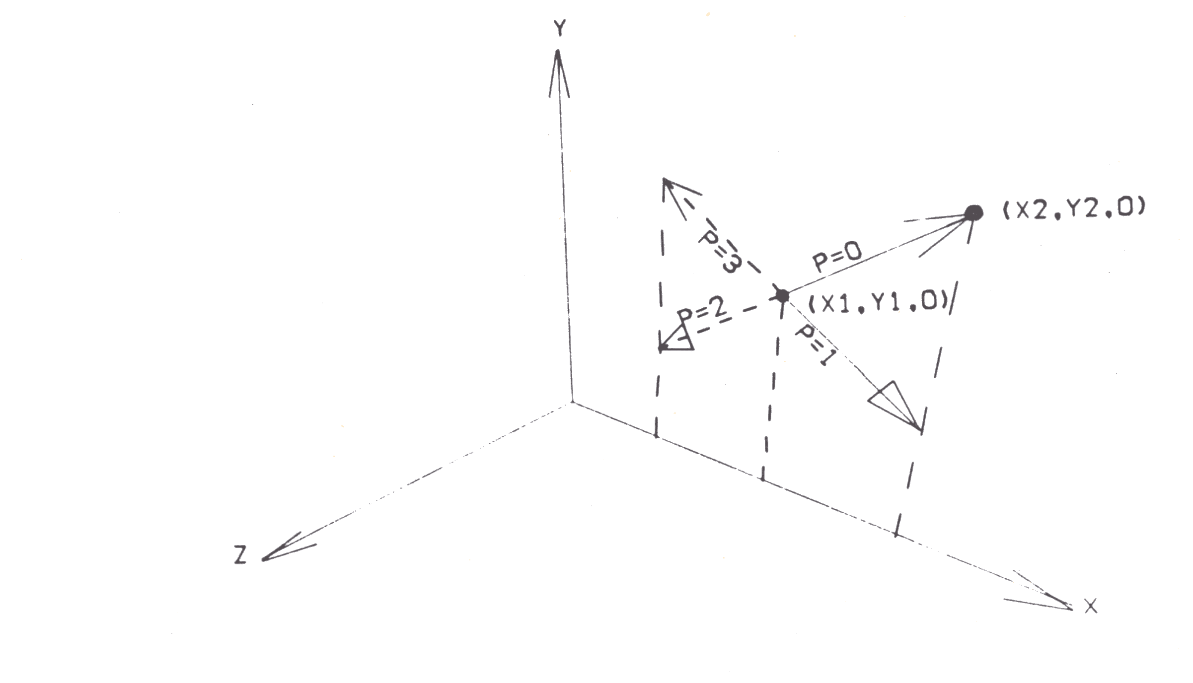
ARROW S ARR P X1 Y1 X2 Y2 HEAD
defines an arrow directed from (X1,Y1,0) to (X2,Y2,0) with a head of length, HEAD. The figure lies in the x-y plane. the use of the parameter, P, is shown in the diagram below.
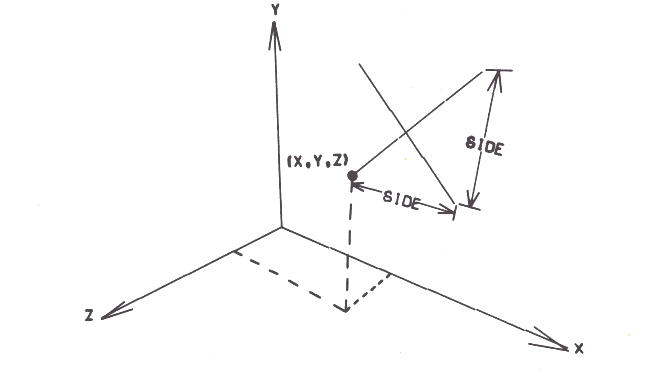
CROSS S ARR * X Y Z SIDE
defines a cross with lower left hand corner a (X,Y,Z) of height and width SIDE. This figure lies in a plane parallel to the x-y plane.
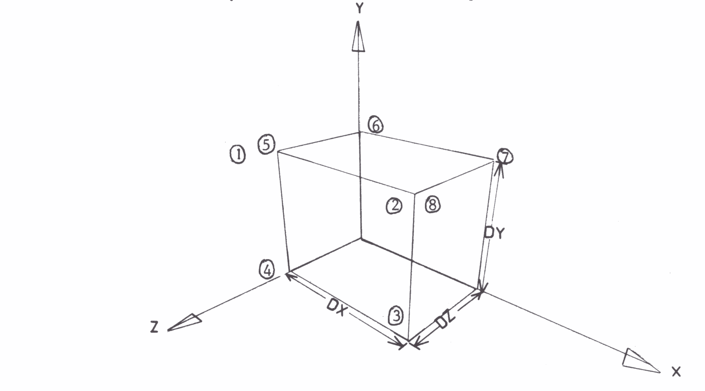
BOX S ARR * DX DY DZ
defines a box with one corner at the origin and sides of length DX, DY and DZ in the positive X, Y and Z directions respectively. The order of points within the array is shown by the circled numbers in the diagram below. If only the top and the front of the box are required, the first 8 points should be transferred into a new array. No more than 8 points should be transferred from a box array except when the whole array is transferred. this is because subarrays are used after the 8th point.
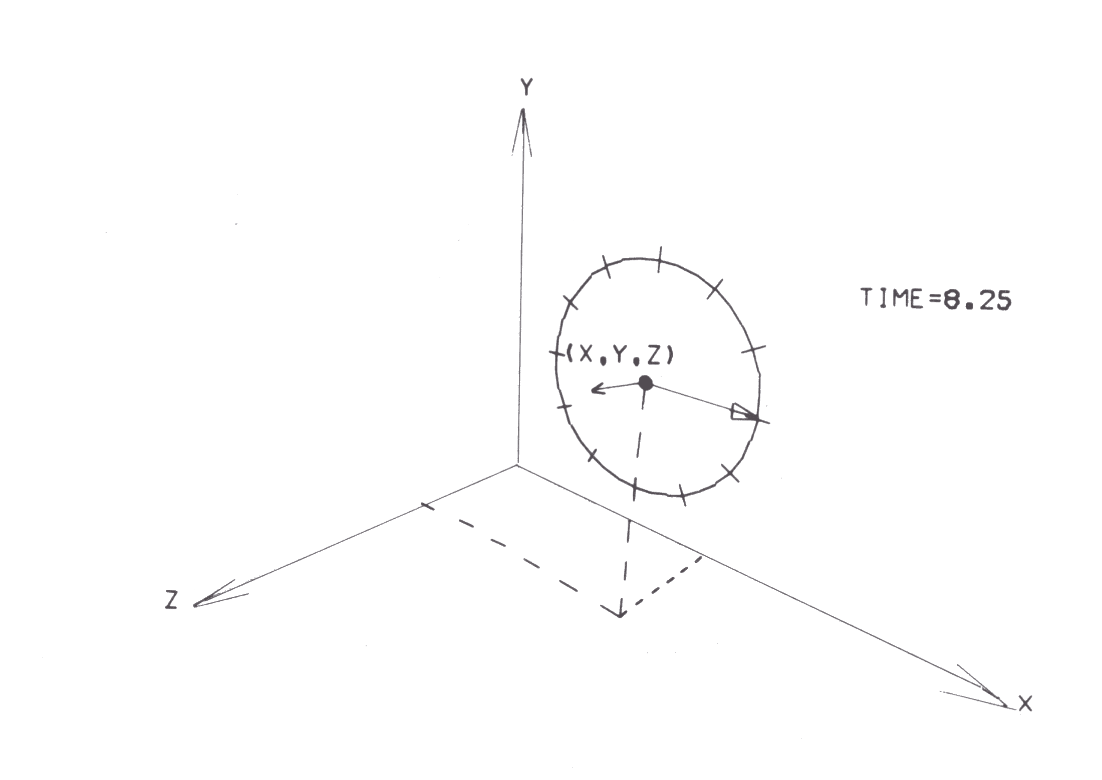
CLOCK S ARR * X Y Z RAD TIME
defines a clock face centred at (X,Y,Z) of radius, RAD, showing the time, TIME. The integer portion of TIME is the hour, and the fraction part is the decimal fraction of an hour. This figure lies in a plane parallel to the x-y plane. Additional figures can be defined out of lines.
SETCV S ARR * X Y Z
defines the first point (X,Y,Z) of a series of points to be connected consecutively by straight lines.
SETLN S ARR * X Y Z
defines the first point (X,Y,Z) of a series of pairs of points which represent a set of unconnected straight lines.
EXPAR S ARR * X Y Z
expands a previously defined SETCV or SETLN array by adding point (X,Y,Z) onto the end. EXPAR can be used as many times as desired, but it should only expand that array which is currently at the end of the stack. SETCV should have at least one EXPAR command following it. SETLN should have an odd number of EXPAR commands following it to make sure that a complete set of pairs of points is defined.
C * * * * * * * * COMMENTS
ERASE S ARR
erases the contents of array ARR of stack S. If ARR is blank or zero the whole stack is erased. This command should be used at the beginning of each new sequence to avoid any carry-over from the previous sequence.
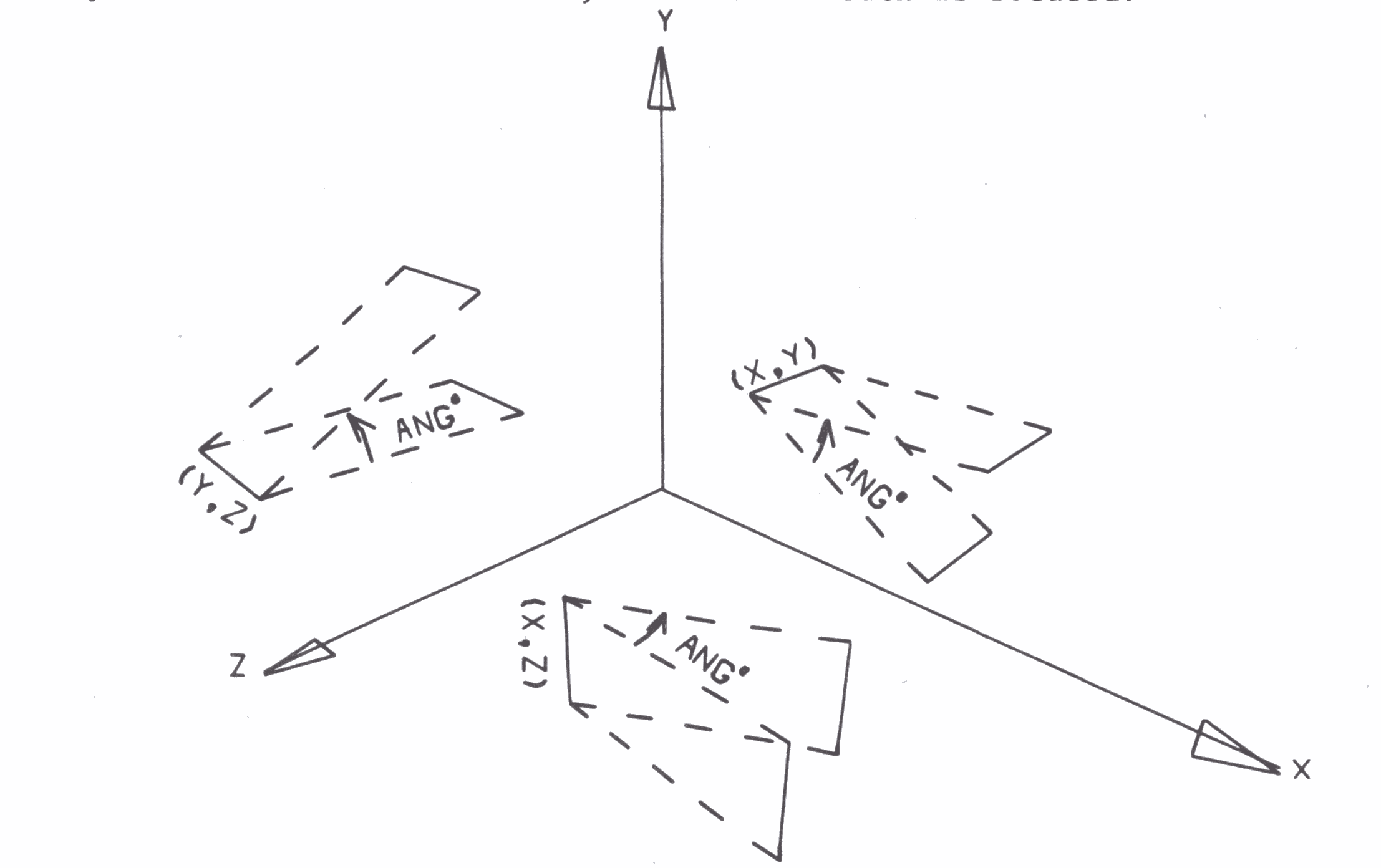
XYROT S ARR * X Y ANG
rotates array ARR of stack S about the line x=X, y=Y by ANG degrees. If ANG is positive, the rotation is counter clockwise as the x-y plane is viewed from the positive Z side. As the rotation is about a line perpendicular to the x-y plane, the Z coordinates are not changed by this rotation. if ARR=0, the entire stack is rotated.
YZROT S ARR * Y Z ANG
rotates array ARR of stack S about the line y=Y, z=Z by ANG degrees. If ANG is positive, the rotation is counter clockwise as the y-z plane is viewed from the positive X side. As the rotation is about a line perpendicular t o the y-z plane, the x coordinates are not changed by this rotation. If ARR=0, the entire stack is rotated.
XZROT S ARR * X Z ANG
rotates array ARR of stack S about the line x=X, z=Z by ANG degrees. If ANG is positive, the rotation is counter clockwise as the x-Z plane is viewed from the positive y side. As the rotation is about a line perpendicular to the x-Z plane, the y coordinates are not changed by this rotation. If ARR=0, the entire stack is rotated.
OFFSET S ARR * DX DY DZ
offsets the points of the array ARR of stack S by DX, DY, DZ in the X, Y and Z directions respectively. DX, DY and DZ can be negative. If ARR=0, the entire stack is offset.
SIZE S ARR * XREF YREF XMAG YMAG
expands or contracts all the points of the array, ARR of stack, S about the reference line, x=XREF, y=YREF. New coordinates are computed by the following relations:
x' = (x-XREF) * XMAG + XREF
y' = (y-YREF) * YMAG + YREF
where (x,y) are the first two coordinates of a point in the array. I XMAG and YMAG are greater than one, the points expand about the reference line; if XMAG and YMAG are less than 1, the points contract about the reference line; if XMAG=YMAG=1, the points are unchanged. If XMAG=YMAG=0, all points are set onto the reference line. As long as XMAG and YMAG are equal, the picture merely changes its size without being distorted. If ARR=0, the entire stack is affected. The Z coordinates are unchanged by this command. To reduce or expand a figure in all three directions, use this in conjunction with ZSIZE.
ZSIZE S ARR * ZREF ZMAG
expands or contracts all the pointers of an array about the reference plane z=ZREF. New Z coordinates are computed by the relation:-
z' = (z - ZREF) *ZMAG + ZREF
where z is the third coordinate of a point in the array. ZMAG obeys the same properties as XMAG and YMAG do. To change the size of an array in three dimensions about the point (XREF, YREF, ZREF) use the SIZE command about x=XREF, y=YREF and the ZSIZE command about z=ZREF.
MOVE STA ARRA * STB ARRB
This command is used within a DO LOOP to move in equal increments, a figure whose initial position is stored in stack STA, array ARRA, to a final position which is stored in stack STB, array ARRB.
If both ARRA and ARRB are zero, the entire stack is moved. The parameter NTIMES from the DO instruction determines the total number of equal increments used. After the loop is executed, the stack STA has been set equal to the original value of STB, and stack STB has been destroyed.
TNSFR SB ARRB P P1 P2 SA ARRA BPT1
transfers points P1 to P2 inclusively from array ARRA, stack SA into array ARRB, stack SB. Point P1 of array ARRA will begin loading into array ARRB, starting at point BPT1. If BPT1 is left blank or set to zero, it is assumed to be 1.
If ARRB is a New Array:-
P = 0 all three coordinates are transferred
P = 1 only x-coordinates are transferred
P = 2 only y-coordinates are transferred
P = 3 only z-coordinates are transferred
If ARRB already exists:-
P = 4 all three coordinates are transferred
P = 5 only x-coordinates are transferred
P = 6 only y-coordinates are transferred
P = 7 only z-coordinates are transferred

P = 9 all coordinates of the points in ARRA are transferred from the given
      starting point to array ARRB until either all the points P1 to P2 are
      transferred, or until the end of the array ARRA is reached, whichever
      occurs first. To transfer the whole of an array of unknown size, a
      fictitiously high value of P2 can therefore be used.
POINT S ARR * X Y Z PT
replace the PTth point of array ARR of stack S with the new point (X,Y,Z). Array ARR should already have been set up.
DUMP S
prints the contents of the 1000 locations of stack S.
LETER S ARR * * * * * * TEXT
adds up to 20 characters of TEXT into stack S, starting with array ARR. The text is placed in column 61 onwards. If less than 20 characters are required, the > sign can be used to terminate the string. The text is then loaded into stack S, beginning in array ARR, with each new character placed into the next consecutive array and offset 1 unit in the positive x-direction. The first character is located with the lower left hand corner at (ARR-1, 0, 0) and the following characters at (ARR, 0), ARR+1, 0 , 0) and so on. All characters lie in the x-y plane (Z=0).
So far we have implied that the arguments in the class 1 and 2 commands are constant values which define the action of the command. However, it is sometimes useful to be able to define a command which can vary in meaning. CAMPER defines a set of 9 variables, V1 to V9, which can be set to a particular value or manipulated by the class 3 commands. It is possible to replace all arguments other than the stack and parameter arguments by one of the nine variables. Due to limitations in the FORTRAN input/output package (the language in which CAMPER is written), it is not possible to write, for example, V1 in a CAMPER command as only numbers are allowed. Most arguments should be small numbers. Therefore V1 to V9 are represented by the numbers 901.0 to 909.0. For example:-
1     6  9 12 4     21 3      31 3
CIRCL1   10 4.0      4.0       3.0
defines a circle centred at (4.0,4.0) and radius 3.0.
1     6  9 12 4     21 3      31 3
CIRCL1   10 4.0      4.0       901.0
defines a circle centred at (4.0,4.0) and radius equal to the current value of the variable V1. arguments greater than 909.0 will be treated as being in error and will halt the program.
The introduction of variables does not, by itself, increase the flexibility of the system by much. However, there are class 3 commands which allow a set of commands to be repeated a number of times. if these commands depend on the current values of variables, it is possible to achieve quite complex picture manipulations with a few CAMPER commands in a loop.
The class 3 commands have the general format
CMND * * VAR OPRND BGIN END
The argument VAR is in the parameter field and therefore must be a single digit. This defines the particular variable to be used in the operation. A variable used in any other argument position will have the usual representation, ie the constants 901.0 to 909.0.
The two parameters BGIN and END decide whether or not this command is to be executed. if V9 is less than the value of BGIN then the command will not be executed. if END is not blank or zero then the command will only be executed if V9 is less than the value of END.
The two parameters BGIN and END decide whether or not this command is to be executed. If V9 is less than the value of BGIN then the command will not be executed. If END is not blank or zero then the command will only be executed if V9 is less than the value of END
In general, V9 is reserved to mean the loop variable. it is therefore sensible never to set V9 except when it is defined by a loop.
The class 3 commands are as follows:-
ADDV * * VAR OPRND BGIN END
places the contents of variable VAR plus OPRND into VAR
SUBV * * VAR OPRND BGIN END
places the contents of variable VAR minus OPRND into VAR
MULTV * * VAR OPRND BGIN END
places the contents of variable VAR times OPRND into VAR
DIVV * * VAR OPRND BGIN END
places the contents of variable VAR divided by OPRND into VAR
SINV * * VAR OPRND BGIN END
places the sine of OPRND degrees into variable VAR
COSV * * VAR OPRND BGIN END
places the cosine of OPRND degrees into variable VAR
SQRTV * * VAR OPRND BGIN END
places the square root of OPRND into variable VAR
EXPV * * VAR OPRND BGIN END
places eOPRND into variable VAR
DO * * * NTIMES
sets up a loop of commands to be repeated NTIMES iterations. The DO loop should not be more than 100 commands in length.
LOOP
defines the end of the group of commands starting with DO which comprises the loop. Loops cannot be nested, ie one must end before another begins.
LOOP
On obeying the DO command initially, the variable V9 is set to 1. Each time the loop command is encountered, the value of V9 is increased by one and the commands immediately following the DO command are executed again. this continues until the value of V9 is equal to NTIMES when the loop command is executed. In this case the next command obeyed is the one following the LOOP command.
RDRAW S ARR P X Y Z PP NODRW
SDRAW S ARR P OVER UP RAD PP NDRAW
Both commands output the perspective trace of the picture contained in array ARR of stack S. If ARR=0, the entire stack is output. In RDRAW, the viewing point is given in Cartesian coordinates as (X,Y,Z). In SDRAW, the viewing point is given in spherical coordinates at OVER degrees from the Z-axis, UP degrees from the x-z plane and a radial distance of RAD from the origin.
The projection plane is located PP units from the viewing point, towards the origin. The figure to be plotted normally lies on the opposite side of the projection plane from the viewing point, since the projected image is then smaller than actual size. If the figure to be plotted lies between the projection plane and the viewing point, the plot will appear larger than actual size. As PP increases, the picture size is magnified, and vice versa. RAD and PP should always be positive. the angles OVER and UP can become negative, if desired.
If NODRW=0, this command is executed, while if NODRW=1 it is ignored. The value of NODRW is usually defined as a variable which changes its value around a loop to start or stop output of this picture.
The parameter P=1 will cause the perspective view of the figure to be tested at the outer border so that any portion of a line lying outside the 9 by 12 cine frame is not drawn. If P=0, no test is done. This feature is quite useful, since the programmer has no prior knowledge of whether the projected lines will spill out of the standard drawing rectangle.
If the solid figure lies within a 10 by 10 by 10 box, a good set of parameters for a 12 by 9 picture window would be OVER=45, UP=35, RAD=26, PP=12, or alternatively X=15, Y=15, Z=15, PP=12.
In the following commands, the 2-D origin referred to is the bottom left hand corner of the plotting area which is normally 12 by 9 in size. The 3-D origin is the location of the (0,0,0) point on the plotting area when the picture is output in perspective on the plotting area.
FRAME
This advances the film by one frame. a new frame is now available for output.
NUORG * * * X Y
This positions the 3-D origin X units over and Y units up from the current 2-D origin. X and Y may be negative if desired. This command is necessary to place the projected picture upon the centre of the plotting surface. Unless NUORG is called the 2-D and 3-D origins are at the same point. It is then likely that the part of the figure in the positive Z direction would spill off the bottom of the plotting area. a good set of values might be X=5, Y=4.
STOP
terminates the CAMPER program and output filemarks on the tape and generates statistics.
SAVE
ESAVE
REPET
These three commands are used to store picture drawing SD4020 instructions which are to be repeated many times. They save a considerable amount of computing time. SAVE begins storing all drawing and frame advance instructions instead of performing them. Approximately 2500 lines can be saved. If this number is exceeded, an error message is printed, and the program stops. Each time SAVE is obeyed, the previous saved commands are destroyed.
The command ESAVE ends the saving process. any further drawing or frame advance commands are obeyed rather than being saved.
The REPET command performs all the SD4020 instructions that have been stored for NTIMES. For example:-
123456789012345678901234567890
SAVE
DRAW 1  0  0.0
DRAW 2  0  0.0
FRAME
ESAVE
DO         96.0
OFSET3  0  0.1      0.1
WDRAW3  01
REPET      1.0
LOOP
This set of commands saves the stationary figures in stacks 1 and 2 and the advance film. For each iteration, the figure in stack 3 is moved and then output with the stationary information on the next frame.
FRAME
This concludes the current frame of film and moves the film ready for output on the next frame.
STOP
stops the program.
CAMRA * * P
If I=1, the 16mm film camera is selected for output.
If I=2, the hardcopy camera is selected for output.
If I=3, both cameras are selected together.
START
This command is only required by the 1906A and has to be the first instruction input to the system. It does in fact start the program.
| Columns | 1-5 | 6 | 7-9 | 10 | 11-20 | 21-30 | 31-40 | 41-50 | 51-60 | 61-80 |
|---|---|---|---|---|---|---|---|---|---|---|
| Class | Name | Stack | Array | Par | Arg1 | Arg2 | Arg3 | Arg4 | Arg5 | Comments |
| 1 | CIRCL | S | ARR | D | X | Y | Z | RAD | ||
| 1 | RECT | S | ARR | X | Y | Z | LNGTH | HGT | ||
| 1 | TRNGL | S | ARR | X | Y | Z | BASE | HGT | ||
| 1 | ARROW | S | ARR | P | X1 | Y1 | X2 | Y2 | HEAD | |
| 1 | SETCV | S | ARR | X | Y | Z | ||||
| 1 | SETLN | S | ARR | X | Y | Z | ||||
| 1 | EXPAR | S | ARR | X | Y | Z | ||||
| 1 | CROSS | S | ARR | X | Y | Z | SIDE | |||
| 1 | BOX | S | ARR | D | DX | DY | DZ | RAD | ||
| 1 | CLOCK | S | ARR | X | Y | Z | RAD | TIME | ||
| 2 | C | COMMENTS | ||||||||
| 2 | ERASE | S | ARR | |||||||
| 2 | XYROT | S | ARR | X | Y | ANG | ||||
| 2 | XZROT | S | ARR | X | Z | ANG | ||||
| 2 | YZROT | S | ARR | Y | Z | ANG | ||||
| 2 | OFSET | S | ARR | DX | DY | DZ | ||||
| 2 | SIZE | S | ARR | XREF | YREF | XMAG | YMAG | |||
| 2 | ZSIZE | S | ARR | ZREF | ZMAG | |||||
| 2 | MOVE | STA | ARRA | STB | ARRB | |||||
| 2 | TNSFR | SB | ARRB | P | P1 | P2 | SA | ARRA | BPT1 | |
| 2 | POINT | S | ARR | X | Y | Z | PT | |||
| 2 | DUMP | S | ||||||||
| 2 | LETER | S | ARR | TEXT | ||||||
| 3 | ADDV | VAR | OPRND | BGIN | END | |||||
| 3 | SUBV | VAR | OPRND | BGIN | END | |||||
| 3 | MULTV | VAR | OPRND | BGIN | END | |||||
| 3 | DIVV | VAR | OPRND | BGIN | END | |||||
| 3 | SINV | VAR | OPRND | BGIN | END | |||||
| 3 | COSV | VAR | OPRND | BGIN | END | |||||
| 3 | EXPV | VAR | OPRND | BGIN | END | |||||
| 3 | SQRTV | VAR | OPRND | BGIN | END | |||||
| 3 | DO | NTIMES | ||||||||
| 3 | LOOP | |||||||||
| 4 | RDRAW | S | ARR | P | X | Y | Z | PP | NODRW | |
| 4 | SDRAW | S | ARR | P | OVER | UP | RAD | PP | NODRW | |
| 4 | FRAME | |||||||||
| 4 | NUORG | X | Y | |||||||
| 4 | STOP | |||||||||
| 4 | SAVE | |||||||||
| 4 | ESAVE | |||||||||
| 4 | REPET | NTIMES | ||||||||
| 4 | CAMRA | P | ||||||||
| 4 | START |
the following characters are already defined in stack 7 when CAMPER is entered.
| Character | Array | Number of Points |
Character | Array | Number of Points |
|---|---|---|---|---|---|
| A | 1 | 8 | U | 21 | 6 |
| B | 2 | 12 | V | 22 | 4 |
| C | 3 | 8 | W | 23 | 6 |
| D | 4 | 8 | X | 24 | 4 |
| E | 5 | 8 | Y | 25 | 6 |
| F | 6 | 6 | Z | 26 | 4 |
| G | 7 | 10 | , | 27 | 6 |
| H | 8 | 6 | . | 28 | 6 |
| I | 9 | 6 | - | 29 | 2 |
| J | 10 | 12 | 0 | 30 | 10 |
| K | 11 | 6 | 1 | 31 | 6 |
| L | 12 | 4 | 2 | 32 | 8 |
| M | 13 | 6 | 3 | 33 | 14 |
| N | 14 | 4 | 4 | 34 | 6 |
| O | 15 | 10 | 5 | 35 | 10 |
| P | 16 | 8 | 6 | 36 | 12 |
| Q | 17 | 12 | 7 | 37 | 4 |
| R | 18 | 14 | 8 | 38 | 16 |
| S | 19 | 14 | 9 | 39 | 12 |
| T | 20 | 4 | space | 40 | 2 |

| FIGURE | LOCATIONS |
|---|---|
| Circle | 112 |
| Circle (Dashed) | 109 |
| Cross | 13 |
| Triangle | 13 |
| Rectangle | 16 |
| Box | 51 |
| Clock | 222 |
| Arrow (Solid Tail, Open Head) | 17 |
| Arrow (Solid tail, Closed Head) | 20 |
| Arrow (Dashed Tail, Open Head) | 47 |
| Arrow (Dashed Tail, Closed Head) | 50 |
| Set Line array (SETLN) | 4 |
| Set Curve Array (SETCV) | 4 |
| Expand Array (EXPAR) | 3 |
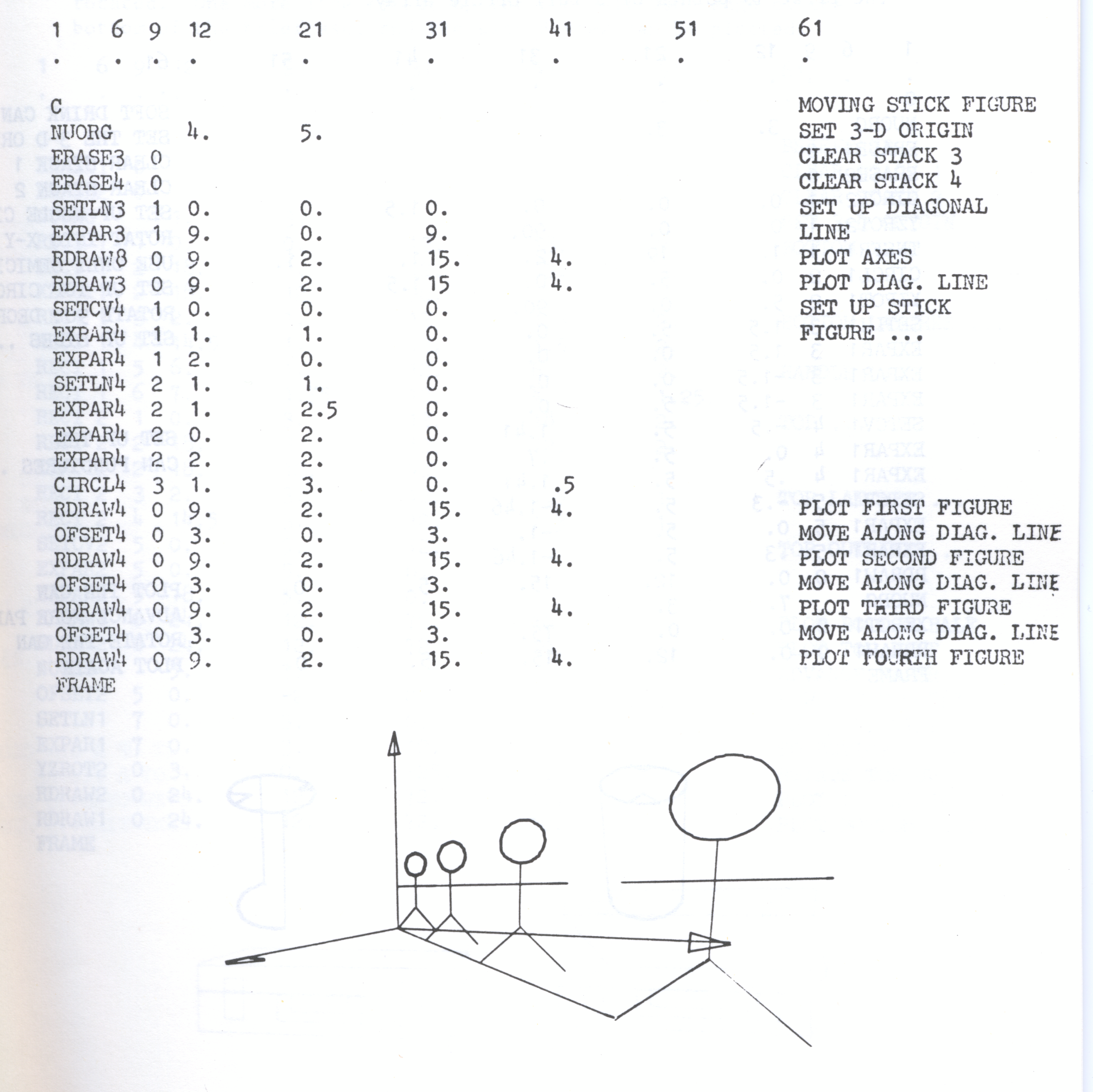
To demonstrate the effect of perspective drawings, a series of views is plotted of a stick figure advancing toward the picture plane. The standard set of axes in stack 8 is used here. A diagonal line is also shown at 45 degrees to the Z axis. The figure is advanced equal distances along the diagonal line and plotted. It appears larger as it approaches the picture plane. in the last view, it s drawn virtually the same size as the actual figure in 3D coordinates (which is 3.5 units high). This means that the picture plane is at about the same distance from the viewing point as the figure.
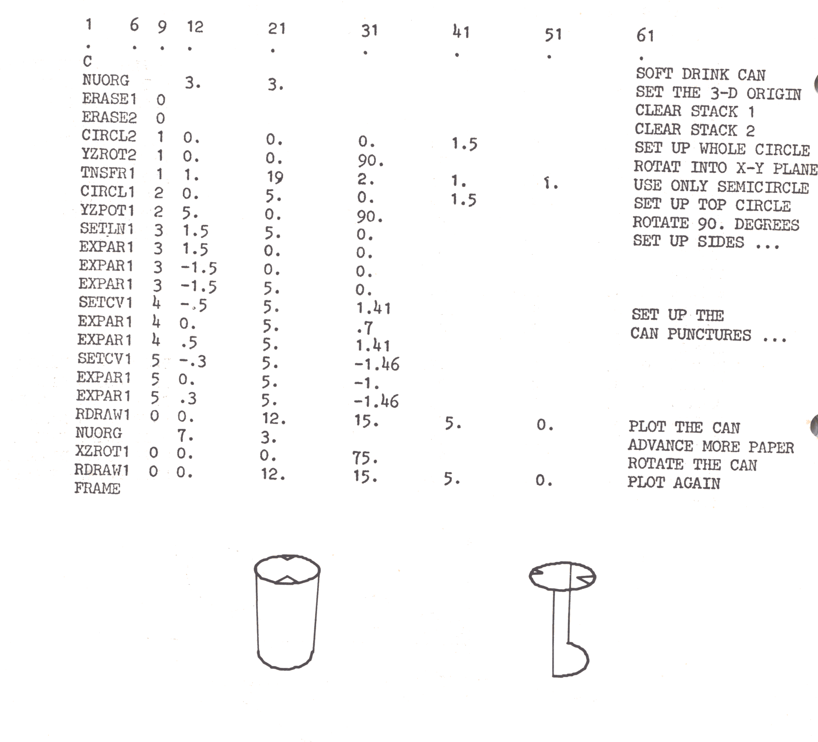
Often a round surface must be depicted in a perspective plot. This is readily handled by showing the edge as a straight line. A soft drink can, for example, can be set up by a circle, a semicircle, 2 puncture marks, and 2 straight lines for the sides. when viewed head-on, this appears quite normal. However, when either the point of view, or the can itself as below is rotated, an absurd picture results. This is because the straight lines actually represent the edge of a continuous surface. In the example below, only the can puncture (arrays 4 and 5 of stack 1) should have been rotated. Notice also that the semicircle was created by transferring the first 19 points of a full circle array.
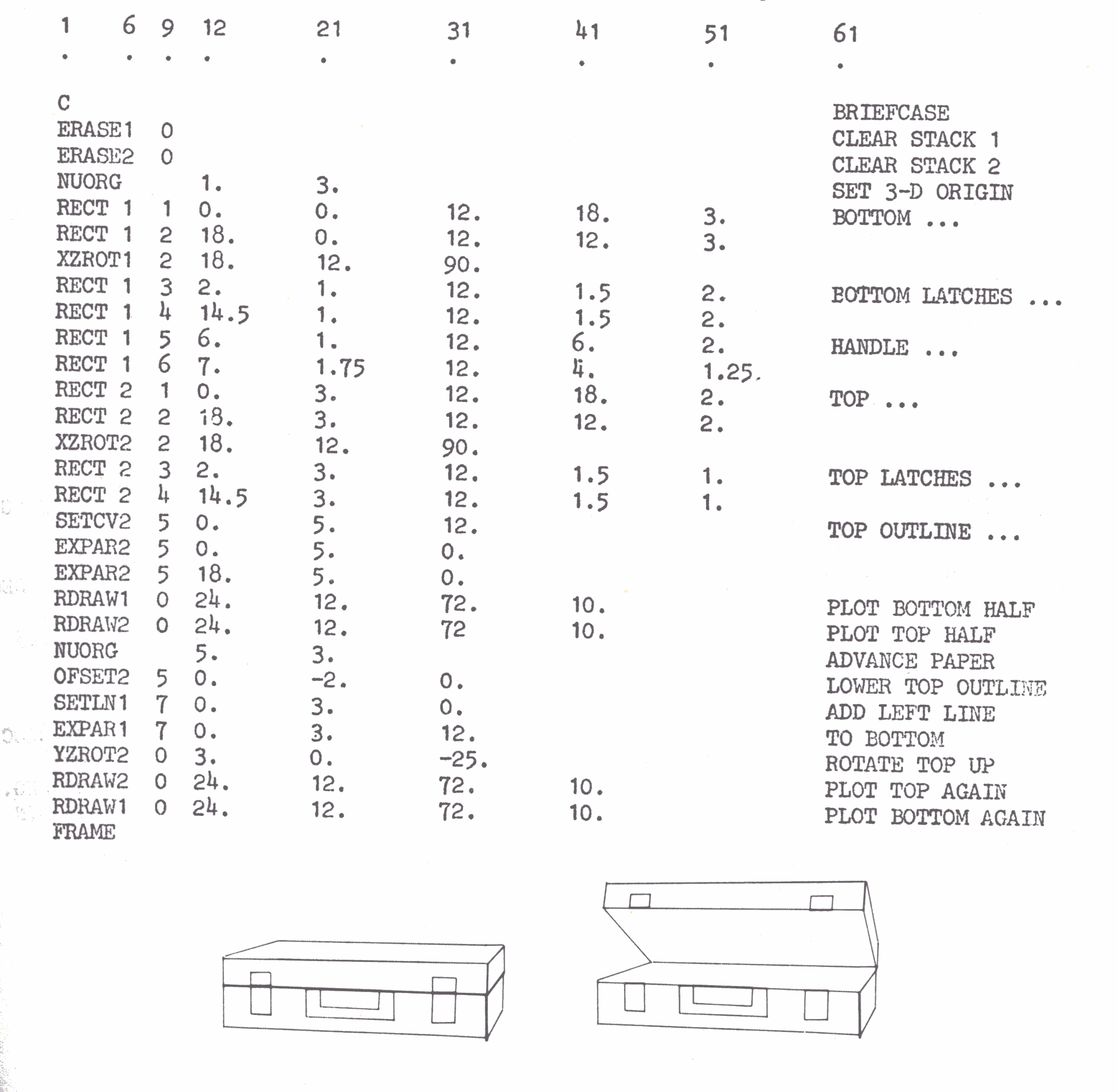
When a moving solid figure is observed from a fixed position, certain of its edges may disappear from view. these are called hidden lines, and unfortunately it is the task of the CAMPER user to suppress them when necessary. Such a case is shown below; a brief case in fact! It is rather simply set up by a series of rectangles and plotted in the closed position. The back and left edges of the top can be seen in this first view. Before the lid can be shown rotated upwards, however, these two lines must be eliminated, and the bottom of the lid must appear. these aims are both accomplished by offsetting those two lines down two units before the lid is rotated. One more line is set up for the left-hand edge of the bottom of the brief case, and the second view can be plotted.
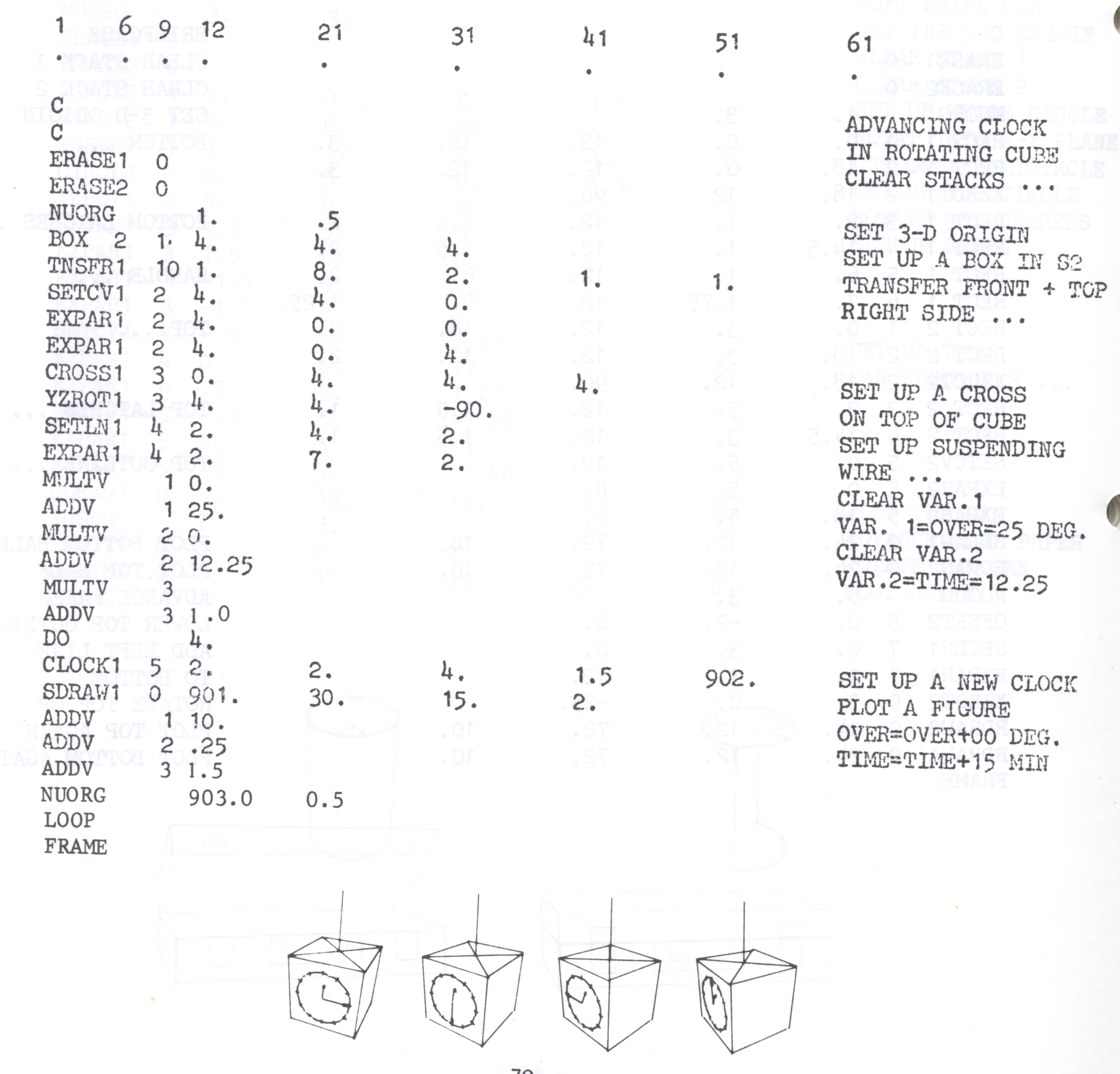
Suppose a clock is mounted on the face of a cube which rotates very slowly. to show this, a box is set up and the first eight points are transferred to plot the front and top planes only. the side plane is et up separately by a SETCV array. A cross is set up and rotated parallel to the XY plane, and a line to its centre serves as a suspending cable. Four views show the clock every 15 minutes. Variable 1 is used for the argument TIME in the CLOCK command. It is incremented by .25 each iteration; this advances the clock hands 1/4 of an hour each time. The rotation could have been achieved by rotating the whole figure, in which case the clock would have been set up parallel to the X-Y plane and rotated a little more for each view. It is slightly easier here to let the figure remain stationary, and simply rotate the point of view. this is accomplished by letting the argument OVER in the command SDRAW increase by 10 degrees for each view.